Generating Cats Using Generative Adversarial Networks and Principal Component Analysis


Aim
This article will provide you with a general framework of a Generative Adversarial Network written using the Keras library. You will be able to use this generic GAN template to train generative models using your own image datasets.
The complete version of the code is available at this Github repository .
Dataset

Imports
from keras.layers import Input, Dense, Reshape, Flatten
from keras.layers.advanced_activations import LeakyReLU
from keras.layers.convolutional import UpSampling2D, Conv2D, MaxPooling2D
from keras.models import Sequential, Model
from keras.optimizers import Adam
from sklearn.utils import shuffle
from sklearn.decomposition import PCA
import matplotlib.pyplot as plt
import numpy as np
import os
from PIL import Image
Using TensorFlow backend
- Keras (I use 2.3.1)
- Tensorflow (I use 1.14.0)
- Sklearn
- Scipy
- Numpy
- Matplotlib
- PIL
- Keract (Optional, for Model Visualization)
Set Parameters
# Folder containing dataset
data_path = r'D:\Downloads\cats-faces-64x64-for-generative-models\cats'

# Dimensions of the images inside the dataset
img_dimensions = (64,64,3)

# Folder where you want to save to model as well as generated samples
Set the dataset_path = r"C:\Users\Vee\Desktop\python\GAN\pca_new"

# How many epochs between saving your model
interval = 10

# How many epochs to run the model
epoch = 500

# How many images to train at one time.
# Ideally this number would be a factor of the size of your dataset
batch = 181

# How many convolutional filters for each convolutional layer of the generator and the discrminator
conv_filters = 64

# Size of kernel used in the convolutional layers
kernel = (5,5)

# Boolean flag, set to True if the data has pngs to remove alpha layer from images
png = False
Create Deep Convolutional GAN Class
- __init __ (self): The class is initialized by defining the dimensions of the input vector as well as the output image. The Generator and Discriminator models get initialized using build_generator() and build_discriminator() .
- build_generator(self): Defines Generator model. There are 5 convolutional layers, upsampling from 8x8x8 to 64x64x3. Gets called when the DCGAN class is initialized.
- build_discriminator(self): Defines Discriminator model. There are 5 convolutional layers, downsampling from 64x64x3 to 1 scalar prediction. Gets called when the DCGAN class is initialized.
- load_data(self): Loads data from user specified file path, data_path Uses PCA to project the image dataset onto a lower dimension as X_Train dataset. Processes image dataset and reshape to 4 dimensions for Y_Train dataset. Gets called in the train() method.
- train(self, epochs, batch_size, save_interval): Trains the Generative Adversarial Network. Each epoch trains the model using the entire dataset split up into chunks defined by batch_size If the epoch is at save_intervalthen the method calls save_imgs() to generate samples and saves the model of the current epoch.
- save_imgs (self, epoch, gen_imgs, y_points): Saves the model and generates prediction samples for a given epoch at the user specified path, Set the dataset_pathEach sample contains 8 generated predictions and 8 training samples.
Initialization
class DCGAN():

    # Initialize parameters, generator, and discriminator models
    def __init__(self):

        # Set dimensions of the output image
        self.img_rows = img_dimensions[0]
        self.img_cols = img_dimensions[1]
        self.channels = img_dimensions[2]
        self.img_shape = (self.img_rows, self.img_cols, self.channels)

        # Set dimensions of the input noise
        self.latent_dim = 512

        # Chose optimizer for the models
        optimizer = Adam(0.0002, 0.5)

        # Build and compile the discriminator
        self.discriminator = self.build_discriminator()
        self.discriminator.compile(loss='binary_crossentropy',
            optimizer=optimizer,
            metrics=['accuracy'])

        # Build the generator
        self.generator = self.build_generator()
        generator = self.generator

        # The generator takes noise as input and generates imgs
        z = Input(shape=(self.latent_dim,))
        img = self.generator(z)

        # For the combined model we will only train the generator
        self.discriminator.trainable = False

        # The discriminator takes generated images as input and determines validity
        valid = self.discriminator(img)

        # The combined model  (stacked generator and discriminator)
        # Trains the generator to fool the discriminator
        self.combined = Model(z, valid)
        self.combined.compile(loss='binary_crossentropy', optimizer=optimizer)
When the DCGAN class is initialized, we define the size of the images the Neural Network should expect from the dataset. This is specified by the Tuple img_dimensions We also define the latent dimensions, which is the size of our input vector generated from PCA. This is specified by the latent_dim integer.
The optimizer we are using for both models is the Adam optimizer. Feel free to experiment with the learning rate and beta values of the optimizer and see what kind of results you get.
The architecture of the Generative Adversarial Network is defined here, with both models using Binary Cross Entropy loss. The choice of Binary Cross Entropy as the loss function is explained here Feel free to experiment with other loss functions but just keep in mind that both models must use the same loss function.
Load Data
class DCGAN():

    # Initialize parameters, generator, and discriminator models
    def __init__(self):

        # Set dimensions of the output image
        self.img_rows = img_dimensions[0]
        self.img_cols = img_dimensions[1]
        self.channels = img_dimensions[2]
        self.img_shape = (self.img_rows, self.img_cols, self.channels)

        # Set dimensions of the input noise
        self.latent_dim = 512

        # Chose optimizer for the models
        optimizer = Adam(0.0002, 0.5)

        # Build and compile the discriminator
        self.discriminator = self.build_discriminator()
        self.discriminator.compile(loss='binary_crossentropy',
            optimizer=optimizer,
            metrics=['accuracy'])

        # Build the generator
        self.generator = self.build_generator()
        generator = self.generator

        # The generator takes noise as input and generates imgs
        z = Input(shape=(self.latent_dim,))
        img = self.generator(z)

        # For the combined model we will only train the generator
        self.discriminator.trainable = False

        # The discriminator takes generated images as input and determines validity
        valid = self.discriminator(img)

        # The combined model  (stacked generator and discriminator)
        # Trains the generator to fool the discriminator
        self.combined = Model(z, valid)
        self.combined.compile(loss='binary_crossentropy', optimizer=optimizer)
The first method we are adding to the DCGAN class is load_data() This will preprocess all images within the user specified path, data_path . This method gets called inside the train() method to load the data before training.
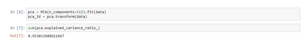
This is where the dataset gets projected onto a lower dimensional space using PCA. The Sklearn PCA method requires the data passed in to be 2 dimensions, so we are squishing the 64x64x3 images to be a 12288 vector. We are also normalizing the data to be between 0 and 1. RGB pixel values range from 0 to 255, so we are dividing the reshaped vector by 255.
Lastly, we shuffle the train() method datasets before returning the two arrays. I wrote the train() method to train the models on the dataset sequentially, incrementing by the batch size each iteration. So it is important to shuffle the dataset to not introduce weird biases relating to the way the dataset is sequentially ordered train() .
Build Generator
 # Define Generator model. There are 5 convolutional filters, upsampling from (8x8x8) to (64x64x3)
    def build_generator(self):

        model = Sequential()

        # Input Layer
        model.add(Dense(8 * 8 * 8, input_dim=self.latent_dim))
        model.add(Reshape((8, 8, 8)))

        # 1st Convolutional Layer
        model.add(Conv2D(conv_filters, kernel_size=kernel, padding="same"))
        model.add(LeakyReLU(alpha=0.2))

        # Upsample the data (8x8 to 16x16)
        model.add(UpSampling2D())

        # 2nd Convolutional Layer
        model.add(Conv2D(conv_filters, kernel_size=kernel, padding="same"))
        model.add(LeakyReLU(alpha=0.2))

        # Upsample the data (16x16 to 32x32)
        model.add(UpSampling2D())

        # 3rd Convolutional Layer
        model.add(Conv2D(conv_filters, kernel_size=kernel, padding="same"))
        model.add(LeakyReLU(alpha=0.2))

        # Upsample the data (32x32 to 64x64)
        model.add(UpSampling2D())

        # 4th Convolutional Layer
        model.add(Conv2D(conv_filters, kernel_size=kernel, padding="same"))
        model.add(LeakyReLU(alpha=0.2))

        # 5th Convolutional Layer (Output Layer)
        model.add(Conv2D(3, kernel_size=kernel, padding="same"))
        model.add(LeakyReLU(alpha=0.2))
        model.summary()

        noise = Input(shape=(self.latent_dim,))
        img = model(noise)

        return Model(noise, img)
The second method we are adding to the DCGAN class is build_generator(). This method is called when the class is first initialized. The architecture of the Generator model is designed here. The model summary will give you a clearer idea on what is actually happening inside this model.
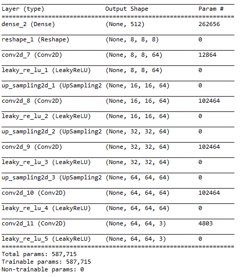
The input of the Generator model is a vector of 512 numbers. The vector is then reshaped to an 8x8x8 tensor. This tensor is then upsampled to 16x16, 32x32, and finally 64x64. The output Convolutional layer contains 3 filters representing the Red, Green, and Blue channels of an RGB image respectively.
Build Discriminator
    The third method we are adding to the DCGAN class is
    def build_discriminator(self):

        model = Sequential()

        # Input Layer
        model.add(Conv2D(conv_filters, kernel_size=kernel, input_shape=self.img_shape,activation = "relu", padding="same"))

        # Downsample the data (64x64 to 32x32)
        model.add(MaxPooling2D(pool_size=(2, 2)))

        # 1st Convolutional Layer
        model.add(Conv2D(conv_filters, kernel_size=kernel, activation='relu', padding="same"))

        # Downsample the data (32x32 to 16x16)
        model.add(MaxPooling2D(pool_size=(2, 2)))

        # 2nd Convolutional Layer
        model.add(Conv2D(conv_filters, kernel_size=kernel, activation='relu', padding="same"))

        # Downsample the data (16x16 to 8x8)
        model.add(MaxPooling2D(pool_size=(2, 2)))

        # 3rd Convolutional Layer
        model.add(Conv2D(conv_filters, kernel_size=kernel, activation='relu', padding="same"))

        # 4th Convolutional Layer
        model.add(Conv2D(conv_filters, kernel_size=kernel, activation='relu', padding="same"))

        # 5th Convolutional Layer
        model.add(Conv2D(conv_filters, kernel_size=kernel, activation='relu', padding="same"))

        model.add(Flatten())

        # Output Layer
        model.add(Dense(1, activation='sigmoid'))

        model.summary()

        img = Input(shape=self.img_shape)
        validity = model(img)

        return Model(img, validity)
The third method we are adding to the DCGAN class is build_discriminator() . This method is called when the class is first initialized. The architecture of the Discriminator model is designed here. The model summary will give you a clearer idea on what is actually happening inside this model.
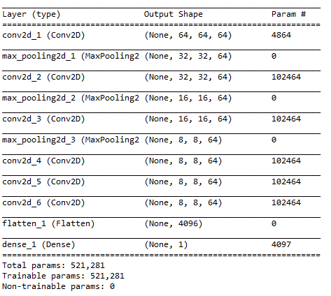
The input of the Discriminator model is a 64x64x3 tensor. The tensor is then downsampled to 32x32, 16x16, and 8x8. This 8x8 tensor is then flattened and passed to the output layer. The final dense layer outputs a single scalar number, representing the prediction of the discriminator model. This prediction represents the confidence of the model in determining if the input image is “real”. A prediction of 1 means the model thinks that the image is from the original dataset. A prediction of 0 means that the model thinks that the image was generated by the Generator model.
Train
 # Train the Generative Adversarial Network
    def train(self, epochs, batch_size, save_interval):

        # Prevent script from crashing from bad user input
        if(epochs <= 0):
            epochs = 1

        if(batch_size <= 0):
            batch_size = 1

        # Load the dataset
        X_train, Y_train = self.load_data()

        # Normalizing data to be between 0 and 1
        Y_train = Y_train/255

        # Adversarial ground truths
        valid = np.ones((batch_size, 1))
        fake = np.zeros((batch_size, 1))

        # Placeholder arrays for Loss function values
        g_loss_epochs = np.zeros((epochs, 1))
        d_loss_epochs = np.zeros((epochs, 1))

        # Training the GAN
        for epoch in range(1, epochs + 1):

            # Initialize indexes for training data
            start = 0
            end = start + batch_size

            # Array to sum up all loss function values
            discriminator_loss_real = []
            discriminator_loss_fake = []
            generator_loss = []

            # Iterate through dataset training one batch at a time
            for i in range(int(len(X_train)/batch_size)):

                # Get batch of images
                imgs = Y_train[start:end]
                noise = X_train[start:end]

                # ---------------------
                #  Train Discriminator
                # ---------------------

                # Make predictions on current batch using generator
                gen_imgs = self.generator.predict(noise)

                # Train the discriminator (real classified as ones and generated as zero)
                d_loss_real = self.discriminator.train_on_batch(imgs, valid)
                d_loss_fake = self.discriminator.train_on_batch(gen_imgs, fake)
                d_loss = 0.5 * np.add(d_loss_real, d_loss_fake)

                # ---------------------
                #  Train Generator
                # ---------------------

                # Train the generator (wants discriminator to mistake images as real)
                g_loss = self.combined.train_on_batch(noise, valid)

                # Add loss for current batch to sum over entire epoch
                discriminator_loss_real.append(d_loss[0])
                discriminator_loss_fake.append(d_loss[1])
                generator_loss.append(g_loss)

                # Increment image indexes
                start = start + batch_size
                end = end + batch_size


            # Get average loss over the entire epoch
            loss_data = [np.average(discriminator_loss_real),np.average(discriminator_loss_fake),np.average(generator_loss)]

            #save loss history
            g_loss_epochs[epoch - 1] = loss_data[2]

            # Average loss of real data classification and fake data accuracy
            d_loss_epochs[epoch - 1] = (loss_data[0] + (1 - loss_data[1])) / 2

            # Print average loss over current epoch
            print ("%d [D loss: %f, acc.: %.2f%%] [G loss: %f]" % (epoch, loss_data[0], loss_data[1]*100, loss_data[2]))

            # If epoch is at intervale, save model and generate image samples
            if epoch % save_interval == 0:

                # Select 8 random indexes
                idx = np.random.randint(0, X_train.shape[0], 8)
                # Get batch of generated images and training images
                x_points = X_train[idx]
                y_points = Y_train[idx]

                # Plot the predictions next to the training imgaes
                self.save_imgs(epoch, self.generator.predict(x_points), y_points)

        return g_loss_epochs, d_loss_epochs

    # Save the model and generate prediction samples for a given epoch
    def save_imgs(self, epoch, gen_imgs, y_points):

        # Define number of columns and rows
        r, c = 4, 4

        # Placeholder array for MatPlotLib Figure Subplots
        subplots = []

        # Unnormalize data to be between 0 and 255 for RGB image
        gen_imgs = np.array(gen_imgs) * 255
        gen_imgs = gen_imgs.astype(int)
        y_points = np.array(y_points) * 255
        y_points = y_points.astype(int)

        # Create figure with title
        fig = plt.figure(figsize= (40, 40))
        fig.suptitle("Epoch: " + str(epoch), fontsize=65)

        # Initialize counters needed to track indexes across multiple arrays
        img_count = 0;
        index_count = 0;
        y_count = 0;

        # Loop through columns and rows of the figure
        for i in range(1, c+1):
            for j in range(1, r+1):
                # If row is even, plot the predictions
                if(j % 2 == 0):
                    img = gen_imgs[index_count]
                    index_count = index_count + 1
                # If row is odd, plot the training image
                else:
                    img = y_points[y_count]
                    y_count = y_count + 1
                # Add image to figure, add subplot to array
                subplots.append(fig.add_subplot(r, c, img_count + 1))
                plt.imshow(img)
                img_count = img_count + 1

        # Add title to columns of figure
        subplots[0].set_title("Training", fontsize=45)
        subplots[1].set_title("Predicted", fontsize=45)
        subplots[2].set_title("Training", fontsize=45)
        subplots[3].set_title("Predicted", fontsize=45)

        # Save figure to .png image in specified folder
        fig.savefig(Set the dataset_path + "\\epoch_%d.png" % epoch)
        plt.close()

        # save model to .h5 file in specified folder
        self.generator.save(Set the dataset_path + "\\generator" + str(epoch) + ".h5")
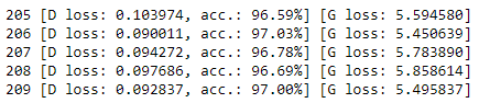
The fourth method we are adding to the DCGAN class is train(). This method will train the network for a specified number of epochs in increments specified by the batch size. When the training completes, the method will return two arrays representing the loss values of both models across every epoch. The loss values can be plotted using Matplotlib.
You should track the loss values and stop training the network if it starts collapsing. The network collapses if one of the models gets close to 0 loss.
If the Generator gets close to 0 loss, then that means the Generator has figured out how to make an image that will fool the discriminator everytime. This will usually result in the Generator only being able to produce one type of image, also known as mode collapse .
If the Discriminator gets close to 0 loss, then that means that the Discriminator has figured out how to distinguish between the training data and generated images very accurately. This will cause the Generator to be unable to continue to learn from the discriminator, also known as the vanishing gradient problem .
To avoid losing our progress when our network collapses, we will save the model every few epochs. The user defined parameter, interval, will determine how often the model gets saved. Every time the current epoch lands on the defined interval, save_imgs() gets called. The method will save an image of some predicted samples to get a snapshot of how good the model was during that epoch.
Save Images
    # Save the model and generate prediction samples for a given epoch
    def save_imgs(self, epoch, gen_imgs, y_points):

        # Define number of columns and rows
        r, c = 4, 4

        # Placeholder array for MatPlotLib Figure Subplots
        subplots = []

        # Unnormalize data to be between 0 and 255 for RGB image
        gen_imgs = np.array(gen_imgs) * 255
        gen_imgs = gen_imgs.astype(int)
        y_points = np.array(y_points) * 255
        y_points = y_points.astype(int)

        # Create figure with title
        fig = plt.figure(figsize= (40, 40))
        fig.suptitle("Epoch: " + str(epoch), fontsize=65)

        # Initialize counters needed to track indexes across multiple arrays
        img_count = 0;
        index_count = 0;
        y_count = 0;

        # Loop through columns and rows of the figure
        for i in range(1, c+1):
            for j in range(1, r+1):
                # If row is even, plot the predictions
                if(j % 2 == 0):
                    img = gen_imgs[index_count]
                    index_count = index_count + 1
                # If row is odd, plot the training image
                else:
                    img = y_points[y_count]
                    y_count = y_count + 1
                # Add image to figure, add subplot to array
                subplots.append(fig.add_subplot(r, c, img_count + 1))
                plt.imshow(img)
                img_count = img_count + 1

        # Add title to columns of figure
        subplots[0].set_title("Training", fontsize=45)
        subplots[1].set_title("Predicted", fontsize=45)
        subplots[2].set_title("Training", fontsize=45)
        subplots[3].set_title("Predicted", fontsize=45)

        # Save figure to .png image in specified folder
        fig.savefig(Set the dataset_path + "\\epoch_%d.png" % epoch)
        plt.close()

        # save model to .h5 file in specified folder
        self.generator.save(Set the dataset_path + "\\generator" + str(epoch) + ".h5")
The fifth and last method we are adding to the DCGAN class is save_imgs() . This method will save the model at the current epoch and plot 8 training images as well as their predicted values.

This method is currently configured to save every 5 epochs. This can be adjusted with the parameter, interval. Frequently saving your model is a good way to track the progress your network is making during the training process.
Initializing The DCGAN Class
We are now done with creating the DCGAN class and ready to train our Generative Adversarial Network. First, we need to create an instance of the class and assign it to a variable.
In [4]:
dcgan = DCGAN()This will initialize the Generator and Discriminator models and print their summaries.
Training The Generative Adversarial Network
Now that we have our DCGAN class object, we just need to call the train() method to start training. With this script, you should generally pick a high number of epochs for training and track the loss values throughout the process. If the network starts collapsing, then stop the training early and check the generated samples to figure out which model was the best performing one.
Train() method returns two arrays containing the loss values of the two models throughout training. We will assign these values to g_loss, and d_loss and plot them.
In [5]:
g_loss, d_loss = dcgan.train(epochs=epoch, batch_size=batch, save_interval=interval)1 [D loss: 0.680393, acc.: 61.54%] [G loss: 0.732704] 2 [D loss: 0.654482, acc.: 60.98%] [G loss: 0.835647] 3 [D loss: 0.680507, acc.: 59.27%] [G loss: 0.832127] 4 [D loss: 0.667612, acc.: 61.23%] [G loss: 0.890128]
5 [D loss: 0.678923, acc.: 57.80%] [G loss: 0.878026]
6 [D loss: 0.669563, acc.: 59.07%] [G loss: 0.857507]
7 [D loss: 0.674293, acc.: 59.85%] [G loss: 0.880131]
8 [D loss: 0.667477, acc.: 58.76%] [G loss: 0.876913]
9 [D loss: 0.663820, acc.: 59.30%] [G loss: 0.891338]
10 [D loss: 0.659955, acc.: 59.45%] [G loss: 0.909291]
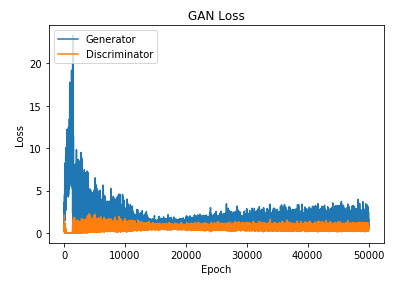
Plot Loss
plt.plot(g_loss)
plt.plot(d_loss)
plt.title('GAN Loss')
plt.ylabel('Loss')
plt.xlabel('Epoch')
plt.legend(['Generator', 'Discriminator'], loc='upper left')
plt.show()
Conclusion
This article provides you with a general framework of training a Generative Adversarial Network using Keras. You will be able to create your own generative models with your own datasets using this script. The full version of this code can be found here. The script is currently configured for 64×64 images.If you want to train using datasets with images of a different size, you will need to adjust the img_dimensions parameter and adjust the amount UpSampling2D and MaxPooling2D layers accordingly.
Once you have trained a model you are satisfied with, you can use the PCA GAN Inference script to generate outputs and analyze your results. This script will also provide you with code to create GIFs of walking through the latent space of the Generator model such as the ones provided at the beginning of the article.
You can also use the Model Visualization script to get a look at what is happening inside each convolutional layer when your modelmakes a prediction.
